While deep reinforcement learning has been shown to be effective in a variety of domains, it suffers from
the same problems as other machine learning methods: it is difficult to interpret and it is difficult to
guarantee that it is behaving correctly. In this article, I present my efforts in reproducing the results of the
paper "Verifiable Reinforcement Learning via Policy Extraction"
The code accompanying this article can be found here.
Background
Reinforcement Learning is gaining increasing importance in safety-critical domains, necessitating the ability to verify that the agent is behaving correctly. This is especially important in domains where the agent is interacting with the real world, such as self-driving cars, air traffic control, and robotics. Unlike playing a game of Go, failure in these real-world scenarios can incur significantly higher perhaps even unacceptable costs. So while there are approaches that aim to teach RL agents safe behavior we would optimally like to be able to demonstrate that our agent never fails.
Even though there is work
Training the oracle
As we will see later for our verification algorithm to work we need to have a functional description of
the state dynamics f(s) of our environment. While the authors are also able to verify other properties such as
robustness in environments where that is not the case such as Atari Pong, we will here only focus on the Toy
Pong environment where we can easily compute the state dynamics.
The environment is a one-player version of the Atari Pong where the player controls a paddle and the opponent is simply a wall. The paddle can move left or right and the ball bounces off the walls and the paddle. The goal is to keep the ball in play for as long as possible. We can describe the state of the environment at timestep t with the following vector:
-
x_p horizontal position of the paddle -
x_b x coordinate of the ball -
y_b y coordinate of the ball -
v_x x velocity of the ball -
v_y y velocity of the ball
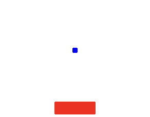
The ball starts at the center of the screen and is initialized with a random velocity
in both the x and the y direction with a magnitude between 1 and 2. The paddle starts at the center bottom of
the
screen and can be controlled via the actions {left, right, stay}.
The speed of the paddle is not given, so I initially assumed it to be 1. However, after some experimentation, I
quickly learned that this makes the game impossible to play perfectly as there are many cases where the ball is
too
fast to catch no matter what the controller does. A quick calculation shows that the paddle's speed needs to be
at least 1.5.
Having the environment
set up we now would like to train an oracle that can play the game perfectly. While the
authors used a generic policy gradient
for training a DNN policy I decided to go directly for the stable baselines 3 PPO implementation as it
is a good starter for Deep RL. Usually it is enough in RL for an agent to achieve a very high reward so training
even this state-of-the-art algorithm to play perfectly
🐍 VIPER
One naive way of approaching the distillation challenge would be to train our decision tree to predict the
action of the oracle given the states of all trajectories in the training set. This, however, turns out to yield
poor
results because the decision tree is not able to generalize to unseen states. This is because mo matter how good
our
action classification accuracy is on the training set, the decision tree will likely end up
in a state where it has never seen before. This is especially true for stochastic environments. DAgger
The VIPER algorithm is based on DAgger but adds one important insight: Not all states in a game are equally important to its outcome. In the figure below for instance we can see that on the left side, the ball is moving away from the paddle so the next action is not consequential for the overall return. On the right side however it is crucial for the paddle to move to the right in order to keep the ball in play. We can use this insight to weight state action pairs by their importance for the overall return. But how do we know which states are critical and which are not?
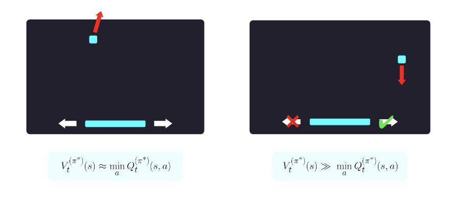
For this, we can leverage the Q-function of the oracle
The sample weights can be obtained directly from our stable baselines oracle policy like so. Now we have all the components to build and analyze the VIPER algorithm. The code below is a simplified snippet from the repository with comments to explain each step:
While I was able to train a decision tree to play perfectly on both CartPole and ToyPong there are a few things to note:
- The only specification w.r.t. to the tree classifier in the paper is that they use the CART algorithm. I found the default Gini coefficient to perform slightly worse than splitting based on entropy.
- For ToyPong my tree ended up much larger than the one reported by the authors (587 vs 61 leaf nodes). I only later realized that in their setup the x position of the ball is likely randomized which would lead to a much more diverse dataset and thus prevents overfitting.
- Pruning helps limit the tree size and can even improve performance as it regularizes the tree.
Differences to DAgger
VIPER extends DAgger with the q-sampling trick, but it also changes the training schedule by only letting the oracle play in the first iteration while DAgger gradually reduces the participation of the oracle in each run. It is thus very easy to modify the above code to work like DAgger, and I was able to verify that both changes lead to better performance.
Verifying Correctness
We now have a DNN policy and a decision tree that both achieve a maximum reward on our ToyPong game. Now we want to verify that there is no edge case that would make our controller lose. This was the hardest part of the implementation and to show why it will help to have a look at the relevant section of the paper:
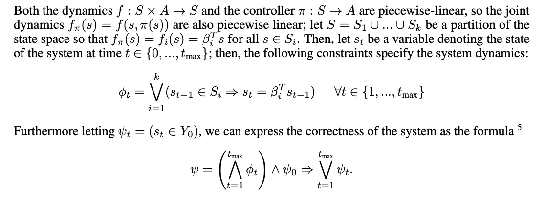
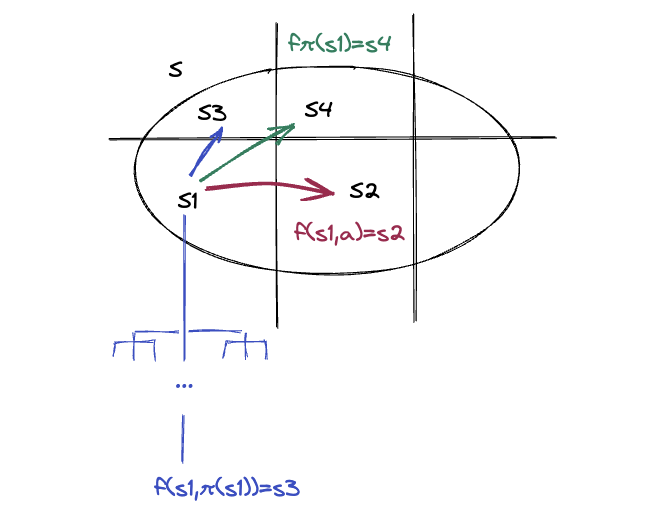
So the idea is that because the joint dynamics $f_{\pi}(s)$ are piecewise linear function we can use the linear programming algorithm to find
exceptions to an equation that says that after at most $ t_{max} $ time steps we always end up in a safe state $
Y_0 $. To better understand the point about the piecewise linearity you can look at the figure below. Decision
trees partition their input space into regions and each region is associated with a leaf node, i.e. action. The
same can be said for the state dynamics which would for instance tell you that within the box the ball keeps
moving while at each wall it bounces back. So if you come up with the right partitioning you
can essentially write the joint dynamics as $f_{\pi}(s) = \beta_i^T s$ where each $\beta_i$ is a vector that
encodes the next state of the system using the controller and system dynamics. Each $ \phi_t $ in the above
program then captures the fact that if we are in one of the state partitions the transition to the next state
will
be governed by the corresponding $\beta_i$
But how do you programmatically build the correct partition and $ \beta $ from the decision tree? At first this question seemed stunningly hard until I realized that there is a straight-forward solution that was probably cut from the paper since it would have only complicated the equations. The trick is to split each expression in $ \phi_t $ into a controller and a system part. The controller part only controls $ s_t[0] $, i.e. the paddle, and the system equations, which have to be specified manually, the rest.
The full correctness check then comes out at less than 300 lines of code with comments. It uses the theorem prover z3 to show that the $ \neg \psi $ is unsatisfiable, i.e. there is no counter example to the safety property. Since my decision tree is considerably larger than the one in the paper the check takes about 38 seconds to run on my 2021 M1 MacBook Pro.
Reflections
The authors of the paper set out and deliver on the very ambitious goal of building a controller that does not only prioritize safety but in fact guarantees it. They also verify other safety properties such as stability and robustness on more environments that were not covered here. However, their verification approach requires the very strong assumption that we have the precise system dynamics as a piecewise linear function. In addition to that the environments are simple enough that we can train a perfect oracle policy that can be distilled into a decision tree. It is therefore an open question what the boundaries of this approach are, i.e. at what point is the difference in DNN policy and DT just big enough so that we cannot distill a perfect DT?
Overall, I greatly enjoyed studying and implementing this paper. The idea of extracting a DT from a DNN policy also has interesting implications for explainable RL agents (if the DT is small enough) and it would be interesting to see if this approach can be extended to more complex environments.