Bayesian methods in RL

A short blog on using Bayesian methods to enable safer reinforcement learning.

Preliminaries

Reinforcement learning (RL) is a powerful approach to train an actor to deal with complex and dynamic environments. However, RL algorithms require a lot of data to learn effective policies, which can limit their practical applications in real-world scenarios. Gathering data can be time-consuming and expensive. Additionally, data collection can sometimes even be dangerous, especially in environments that involve physical robots or complex simulators. An example for this is the training of self-driving cars on public roads. When autonomous vehicles share the roads with human drivers to collect data, a simple mistake by the agent could lead to a dangerous incident. Therefore, there is a growing demand for RL methods that can learn from as few samples as possible while maintaining high performance. This blog will cover a small project on how training an agent in such scenarios can be done in a safer manner.

The Project

The experiments performed use the LAMBDA agent by Yarden As et al. . LAMBDA is a model based agent, and the author's focus is - among other safety related topics -, on sampling efficiency, to increase training safety . Further going down this route, I will introduce a hyperparameter training procedure to LAMBDA. In the paper appendix, the authors mention possible performance improvements when further fine-tuning LAMBDA's hyperparameters. Since LAMBDA already uses a Bayesian world model to create a surrogate world to draw samples from, the hyperparameter optimization approach will also be bayesian. This fits in perfectly with the focus of the paper on reducing the number of iterations needed to optimize the agent.

Background

LAMBDA

LAMBDA is a Bayesian world model based reinfocement learning (RL) agent, that solves tasks in a given virtual environment. The agent can be benchmarked using a suite of safety gym environments. The environment can be modeled as a constrained Markov decision process (CMDP), which can be navigated using learned policies . The reward and cost value functions are modeled using actor, critic and a safety critic neural networks . To increase safety during training and testing, the authors use a Bayesian world model. More specifically, the world model is based on a Recurrent State Space Model (RSSM) . The posterior distribution is obtained using approximations of Bayesian inference (Stochastic Weight Averaging-Gaussian (SWAG) approximation), since exact Bayesian inference is infeasible. This approach allows the authors to draw a set of statistically plausible transition distributions from the world model . These distributions are used to train and guide the exploration and exploitation of the agent.

Bayesian Optimization

Bayesian optimization (BO) is a sequential optimization technique, which is especially present in areas where we do not have any prior information about the function that is to be optimized . For this reason, it is often used in areas like robotics, environmental monitoring or reinfocement learning. What differentiates BO from more conventional optimization algorithms (e.g. gradient descent) is that it is model based. This means that BO uses Bayesian inference to construct a surrogate of the objective function to optimize . The algorithm itself can be divided into two main parts. First, a probabilistic model of the objective function is created, based on prior expert knowledge of the functions behaviour, and additionally all prior function observations in case there are any . Thereafter, a sampling policy, also referred to as the acquisition function, uses the information provided by the probabilistic model to propose a new sampling location, which in the best case maximizes the improvement over the previous best objective function sample. A list of all previous samples is maintained, to which the new observation is added . The optimization procedure now restarts from step one, but the sample list including the latest candidate can now be included in the prior function knowledge . A big advantage of model based optimization methods is the use of a surrogate function. A probabilistic model of the function does not only give us an approximation of the true value at any given input, but also how certain it is in its prediction, based on all previous function evaluations . Exploring areas of high uncertainty provides us with the largest amount of information gain about the objective function . The acquisition function can make use of the uncertainty estimate to more efficiently explore the function space . As a result, we can find function optima fast, using only a small amount of function samples. This is one of the main reasons why BO has gained popularity in the field of hyperparameter tuning in recent years .

In this seminar project, the expected improvement (EI) acquisition function is used as a sampling policy . In the next section, I will go into further detail about the definition of said policy. Furthermore, a Gaussian process is used as a probabilistic model. You can find more in-depth information about Gaussian processes (GP) in the section thereafter (here).

The Expected Improvement Acquisition Function

In the hyperparameter optimization context, many sampling policies are based on the concept of maximizing the probability of an arbitrary point $\bold{x}$ of the black box function $f$ improving upon the value $f(\bold{x})$ of the previous best point $\bold{x}^+$. \max P(f(\bold{x})) \geq f(\bold{x^+}) + \epsilon_n) By varying the parameter $\epsilon_n$, we can control the trade off between exporation and exploitation. It is common to adjust $\epsilon_n$ during the optimization process, such that we ideally explore the function space in the beginning, before exploiting the gained knowledge to find the function optimum. The bold variable $\bold{x}$ denotes that $\bold{x}$ is a vector of hyperparameters.

In the context of Gaussian processes, $f(\bold{x})$ is not a specific function value, but rather a normal distribution over possible function values. The probability of improving upon the previous best observation $f(\bold{x^+})$ is therefore the area under the probability density function centered at the gaussian process mean $\mu$ at point $\bold{x}$, that lies above $f(\bold{x^+})$. From this concept, we can derive our acquisition function. The expected improvement acquisition function we use in our optimization procedure is defined as follows in . EI(\bold{x}) = (\mu(\bold{x}) - f(\bold{x^+}) - \xi) \Phi(Z) + \sigma \phi(Z) where $\phi$ denotes the normal probability density function and $\Phi$ the normal cumulative density function, with Z = \left( \frac{\mu(\bold{x}) - f(\bold{x^+}) - \xi}{\sigma(\bold{x})} \right). $\xi$ here fullfills the same role as $\epsilon_n$ previously, by artificially increasing the value of the previous best sample. A more in-depth derivation of this acquisition function can be found in the original paper , or in a visually more intuitive way in this article .

The Gaussian Process

A Gaussian process (GP) is a collection of infinitely many random variables, where all variables of any finite subset have a joint Gaussian distribution . More intuitively, it can be seen as a distribution over continuous functions . This concept is commonly used to model non-linear relationships between noisy samples. If we want to find an optimum of an unknown function, we can probe the function at certain input locations and record the received observations. We can use a GP to fit a collection of possible functions to the collected data points. The benefit of using a GP in such situations is that it allows us to analytically derive the mean function and the covariances of the measured values . While the mean effectively provides us with an approximation of the objective, the covariances can be seen as a measure of uncertainty in the estimation at any point in function space .

While analytically deriving the mean and variances of a GP is certainly viable for smaller use cases, the performace scales quite poorly. For this reason, oftentimes stochastical approximation methods are used to approximate GPs, similarly to the SWAG algorithm used for LAMBDA . For this project, the simpler analytical solution provided by the BoTorch-library is sufficient.

Implementation

The BO algorithm is implemented in an offline fashion, similarly to the one presented in . In each iteration, the agent is retrained using the new parameters as chosen by the acquisition function. For this project, I chose to optimize the two hyperparameters lambda_ and discount. The library used to implement the Gaussian process and the acquisition function is BoTorch , as it is specifically designed for Bayesian optimization. Another article visualizing the BO procedure can be found here .

The Algorithm

# Pseudo code implementation of the BO Procedure # Number of BO iterations n_iterations = 24 # Lists of hyperparameters to optimize and their respective bounds hyperparameters = [...] bounds = [...] # To avoid a cold start, it is common to start out with a small number of samples samples_x = [...] # = Hyperparameters samples_y = [...] # = Agent scores for i in range(n_iterations): # Feed the GP with all previous objective function samples gp = GaussianProcess(samples_x, samples_y) # Define acquisition function ei = ExpectedImprovement(gp, samples_y.min()) # Optimize EI, retrieve optimal next sampling location (next set of hyperparameters) x_new = optimize_acquisition_function(ei, bounds) agent = LAMBDA() # Train the agent with the new set of hyperparameters trained_agent = train(agent, x_new) # x_new: set of new hyperparameters # Evaluate the agent to get the agents score y_new = evaluate(trained_agent) # Add the new samples to the list of all samples samples_x.append(x_new) sampley_y.append(y_new)

Experiment Setup

To demonstrate the optimization process of the LAMBDA-agent, we will optimize the two hyperparameters lambda_ ($\lambda$) and discount ($d$). These parameters can be found in the critic model of the agent and therefore could have a significant impact on the agents performance. The performance metrics used here are the average undiscounted episodic reward return $\hat{J}(\pi)$, the average undiscounted episodic cost return $\hat{J}_c(\pi)$, and the normalized sum of costs during training (or cost regret) $\rho_c(\pi)$, as defined in .

First Results

For the first test run, I defined the objective function to optimize as $\hat{J}_c(\pi) + \rho_c(\pi)$. Minimizing this function minimizes the cost return of the agent, during training and testing. The reward is ignored for now. In the following interactive figure you can click through the gaussian process mean after each consecutive sample.

Figure 1. The Gaussian process mean, after one to twenty-four samples of the objective function $f(\lambda, d)$. White markers denote already observed objective function samples, the red marker the pending sampling location. A higher function value results in brighter (yellow) color, a lower function value in darker (blue) color. Use the buttons to see how the mean more and more adapts to the ground truth.

We can see that in this example, the minimum of the objective function is found relatively quickly, only after taking a few samples. Let us now take a look at the performance of the agent trained on the best found hyperparameters. The following plot shows the average reward return, average cost return and the cost regret.

Figure 2. The best agent of the first optimization attempt.

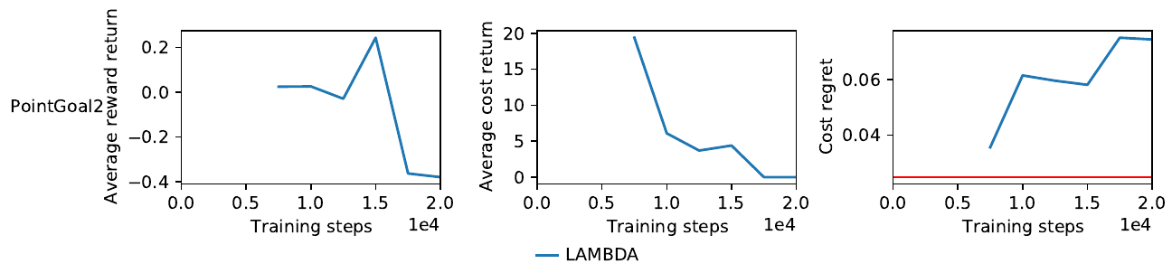
Since we did not include the reward return in the objective function, it is not being optimized. While the average cost return is decreasing with more training steps, as expected, the cost regret is actually rising. The reason why this is happening could be the small magnitude of the measurement when compared to the average cost return. Furthermore, you might notice the smaller number of training steps when compared to the experiments in the paper. We will discuss the reason for this in the last section. For now, we need to improve the objective function.

Second attempt Results

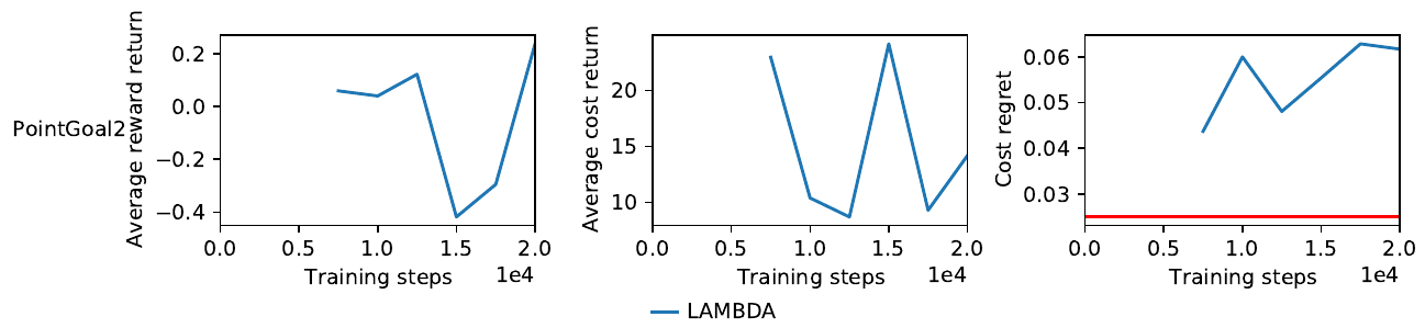
We will now alter the objective function to include the average undiscounted episodic reward return, and futhermore to try to balance out the differences in magnitude by multiplying the cost regret with a constant factor. The latter will hopefully minimize the cost during training. We obtain $\min \hat{J}(\pi) + \hat{J}_c(\pi) + 100 \cdot \rho_c(\pi)$. The optimization process can be seen in the following figure.

Figure 3. The Gaussian process mean, after one to twenty-two samples of the objective function $f(\lambda, d)$.

We observe two minima found by the optimization procedure. Figure 4 shows the performance metrics of the best agent again. The average reward return is now actually improving, while the cost return seems to decrease. Unfortunately, the cost return is unaffected by the increased objective function weight. We note that, while looking better then the first attempt, there is still not a noticable performance improvement. I attribute this fact to several problems, which we will discuss in the next section.

Figure 4. The best agent of the second optimization attempt.

Problems and Prospect

Training LAMBDA is computationally expensive. However, the present experiments are limited by insufficient resources, resulting in a prolonged optimization process of approximately three days to obtain 20 samples. The number of training steps and epochs is already significantly reduced when compared to the paper, which certainly affects the accuracy and representability of the results obtained. When comparing the results of this experiment to the paper results, it becomes apparent that a lot longer training times are needed for the results to stabilize and potential performance benefits to materialize. For this reason, future experiments should be performed on a more capable system, to verify if the implemented optimization procedure works as intended. This would furthermore enable the exploration of more elaborate objective functions than the one used here.

Furthermore, the current implementation of the BO optimization procedure can be numerically instable in some cases. This shows in some of the GP mean plots as aprupt color gradient changes. A stochastic approximation of the exact GP model could help here.

Lastly, more representative results, achieved through longer training times, could also be compared to results achieved using a gradient descent based optimization algorithm, to demonstrate the increased sampling efficiency.

Unfortunately, due to time constraints, I was not able to further explore these suggestions. Despite some problems and road blocks in this project, I learned a lot about Gaussian processes, Bayesian optimization and reinforcement learning.